Appendix A: Optimizing data filling via Vectorization

If you’re too busy to read the chapter, this is basically it!

Appendix prerequisites: Python imports

Before running any code blocks in the following appendix, please ensure you have the necessary Python packages installed via the following code block:

%pip install pandas
%pip install numpy

A.0. Preface: motivating vectorization

In our running examples with GDP data, we’ve typically dealt with datasets that are fairly small by data science standards (~1000 rows or less).

Modern personal machines and shared computing resources (like Stanford’s Sherlock) are ridiculously powerful, and they can quickly chew through almost any code that you write - even if it has zero optimization.

But what happens if you’re dealing with truly massive datasets with hundreds of thousands of rows? With such datasets, code runtime can actually become a constraint on research progression and completion if processing scripts are written suboptimally.

Although the defintion of optimal code and the processing of writing it varies with context, here we’re going to learn a technique that can be applied in many situations: vectorization.

A.1. What, why, when, and how to vectorize

DISCUSSION 1: DEFINING VECTORIZATION

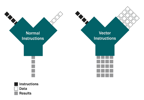
A natural first question to ask is, what is vectorizing/vectorization? You may have heard of vectors before in a mathematics class, where vectors are a series of ordered values like this: [3, 2, 5] or [4, 7, 11, 8].

In computer science, vectorization is a technique related to the mathematical definition of a vector - it’s the process of converting an algorithm from a scalar implementation (which performs operations on, at most, a pair of operands at once) to a vectorized one (which performs operations on a series of values at once). For a quick example:

The processing of a scalar implementation of the instruction, “add two to every element in this list,” would look like:

input: [3, 2, 5] → [3 + 2 = 5, 2, 5] → [5, 2 + 2 = 4, 5] → [5, 4, 5 + 2 = 7] → output: [5, 4, 7]

while the processing of a vectorized implementation of the same instruction would look like:

input: [3, 2, 5] → [3 + 2 = 5, 2 + 2 = 4, 5 + 2 = 7] → output: [5, 4, 7]

(where different processors in your machine carry out the ‘+2’ instruction on each element concurrently.)

If the previous example makes sense to you, congratulations! You understand vectorization. Feel free to come up with your own quicker working definition (mine is, “make computer do same thing to many things at same time.”

DISCUSSION 2: WHY VECTORIZE?

In Python, (almost) any looped operation can be vectorized, but why do we need vectorization in the first place?

While loops are a wonderful and flexible programatic idiom, they’re also inherently slow due to the dynamically typed nature of Python. What does this mean? Let’s take a look in the context of executing a program:

When you execute a program in Python, Python:

• First goes line-by-line through your code;

• Compiles it into a machine-readable version of itself called bytecod*; and

• Then this bytecode is executed to actually run the program.

Suppose your code has a block where you loop over and perform some operation on the elements in a list. As Python is dynamically typed, it does not know the type of the objects present in the list until it accesses each element.

# nothing about the variable name 'a' denotes the type of the contained value. it could be: 
a = 5
print(type(a)) # an int

a = "vectorization rocks!" 
print(type(a)) # a string 

a = dict({"vectorization" : "rocks!"})
print(type(a)) # a dictionary of strings

For any object in Python, the typing information is stored in the the object itself. Therefore, for each iteration in the loop, Python has to perform a series of overhead operations (like determining element type, resolving scope, checking for invalid operations, etc.) until it can carry out the actual operation you instructed it to. As you might imagine, repeatedly performing these overhead operations on massive datasets results in a significantly increased runtime.

A quick aside: A statically typed programming language like C avoids this recurring overhead cost by compelling programmers to explicitly denote the type of every object you use. But, these languages come with their own drawbacks. For example, if two external libraries provide functionality for the same concept with differently-typed implementations, library users will have to provide their own translation layer to allow the two libraries to interoperate. In Python, no/few such interoperability issues arise:

# both pandas and numpy implement an array-type collection
import pandas as pd
import numpy as np 

# instantiating a numpy array and a pandas Series: 
a = np.array([1, 2, 3, 4])
b = pd.Series([5, 6, 7, 8])

# we can use both array variables at the same time, with no confusion from Python!
print("The conductor says: " + str(a))
print("And then: " + str(b.values))
print("And the band goes: 🎶🎷🎶! 🎶🎹🎶! 🎶🎻🎶!")

The conductor says: [1 2 3 4]
And then: [5 6 7 8]
And the band goes: 🎶🎷🎶! 🎶🎹🎶! 🎶🎻🎶!

DISCUSSION 3: ORDER-DEPENDENCE OF OPERATIONS

As we continue to run through our list of interrogatives, we’ve learned the what and why of vectorization - now it’s time to learn the when!

If you recall, we earlier learned that almost any looped operation in Python can be vectorized. To understand the exceptions, we can first classify all looped operations into two types:

1. Order-dependent operations; and

2. Order-independent operations.

As the names suggest, the required order (or lack thereof) of the iterations of a looped operation determines its eligibility for vectorization. Consider the following example:

# suppose we have a Anthony-Land GDP dataset with some discontinuities: 
gdp_data = [(1990, 45), (1991, 46), (1992, 48), (1993, 52), (1995, 55), (1996, 60), (1997, 63), (1999, 67)] # data for the years 1994 and 1998 are missing! 

# if we want to calculate average % increase in gdp from 1990-1999, we have to fill these gaps first! 
#   fill method: gdp_X = avg. of past four years' GDP measurements. 

# 1994 data fill: 
gdp_data.insert(4, (1994, round((gdp_data[0][1] + gdp_data[1][1] + gdp_data[2][1] + gdp_data[3][1])/4))) 
print("After imputing the 1994 data point:" + str(gdp_data))

# 1998 data fill: 
gdp_data.insert(8, (1998, round((gdp_data[4][1] + gdp_data[5][1] + gdp_data[6][1] + gdp_data[7][1])/4)))
print("After imputing the 1998 data point:" + str(gdp_data))

# avg % increase in gdp: 
percent_increase = []
for i in range(len(gdp_data)): 
    if i != 0: percent_increase.append((gdp_data[i][1] - gdp_data[i-1][1])/gdp_data[i][1])

print ("Average % increase in GDP: " + str(round(sum(percent_increase)/len(percent_increase), 4) * 100))

What if we computed filled the two data points in reverse-order?

# same data: 
gdp_data = [(1990, 45), (1991, 46), (1992, 48), (1993, 52), (1995, 55), (1996, 60), (1997, 63), (1999, 67)] # data for the years 1994 and 1998 are missing! 

# same fill method: gdp_X = avg. of past four years' GDP measurements. 

# 1998 data fill: 
gdp_data.insert(7, (1998, round((gdp_data[3][1] + gdp_data[4][1] + gdp_data[5][1] + gdp_data[6][1])/4)))
print("After imputing the 1998 data point:" + str(gdp_data))

# 1994 data fill: 
gdp_data.insert(4, (1994, round((gdp_data[0][1] + gdp_data[1][1] + gdp_data[2][1] + gdp_data[3][1])/4))) 
print("After imputing the 1994 data point:" + str(gdp_data))

# avg % increase in gdp: 
percent_increase = []
for i in range(len(gdp_data)): 
    if i != 0: percent_increase.append((gdp_data[i][1] - gdp_data[i-1][1])/gdp_data[i][1])

print ("Average % increase in GDP: " + str(round(sum(percent_increase)/len(percent_increase), 4) * 100))

A-ha! As you can see, reversing the order that the datapoints were filled in does change the final resulting figure. This is because filling the 1994 data point first makes a 1994 GDP value available as a sample datapoint for imputing the 1998 GDP value, whereas reversing the order of imputation does not.

As such, the operation we just performed is order-dependent (i.e., the final result is contingent upon the order in which any sub-operations are performed) and ineligible for vectorization. Reason being, when an operation is vectorized, Python provides no constraints on the order in which the sub-operations are carried out.

Vectorized operations are to sets, as scalar looped operations are to lists!

Expanding upon our “add 2 to every element in this list” example from before, suppose our input now was much longer: $[3, 2, 5, 4, 6, 11, 14, 8, 1, 37, … (100,000 \text{ more numbers}) …, 24, 2].$ Since our computer likely does not have enough processing units to add 2 to every element concurrently, it’ll perform the vectorized operation in chunks. We can’t guarantee that the first chunk of say, 1000 inputs, coincides with the first 1000 elements in the list.

But, in cases like these, where the final result will be independent of the order of the sub-operations, this random chunking is totally fine! And for that reason, we say order-independent operations can be vectorized.

Note: Determining order-independence (or lack thereof) for any particular operation is a nonstandardized task, but reference to other objects being changed by the same loop is a usually a good sign that order-dependence is present. When in doubt, work with a subset of your data and try switching up the processing order of the loop! Does the result change?

DISCUSSION 4: VECTORIZATION TOOLS

Now that we’ve understood the theory, it’s time to tackle the practice! Here are the relevant tools:

• Libraries:

  • Pandas - the premier Python package for importing, wrangling, and manipulating tabular data.

  • NumPy - Python’s fundamental package for scientific computing, but useful for vectorization due to its vectorization-optimized ndarray.
    
    

• Timer:

  • %timeit - in IPython and Jupyter Notebooks, simply call the magic command ‘%timeit’ suffixed with a function name, and Python will repeatedly run and time the function’s execution to generate runtime statistics.
    
    

• Other useful resources (not used here):

  • line_profiler - an external magic command (requires pip install) which offers a more verbose runtime analysis, including line-by-line hit counts, time per hit, and % total time spent on a line.

  • Cython - yet another external magic command which converts Python code into more loop-friendly C code and supports use of C functions and declaring C types.

(Note on magic commands: Magic commands are those suffixed by the ‘%’ symbol in IPython or Jupyter Notebooks. If you’re using Python through a local installation or IDE, packaged versions of the same tools exist for your import and use.)

A.2. Vectorization in action

CODING EXERCISE: VECTORIZATION - DATA IMPORT

With our tools in hand, let’s go try some vectorization!

# required imports: 
import pandas as pd            # use: data intake and wranglnig
import numpy as np             # use: computing and data structures
import os                      # use: file access and management 

""" BINDER USERS: """
# uncomment: song_df = pd.read_csv('./sample_datasets/unpopular_songs.csv', encoding='utf-8')

""" COLAB USERS: """
# !mkdir data # create a '/data' directory if one doesn't already exist
!wget -P data/ https://raw.githubusercontent.com/roflauren-roflauren/GearUp-MessyData/main/fall_2022/sample_datasets/unpopular_songs.csv # retrieve the dataset from remote storage on GitHub
song_df = pd.read_csv("data/unpopular_songs.csv", encoding='utf-8')

For our vectorization exercises, we’re going to be taking a quick break from GDP data and instead we’ll be using this dataset which contains information about more than 10,000 of the most unpopular songs on Spotify. This information includes the track name, artist, ID, and more subjective measures like danceability, energy, etc.

# a quick view into our data: 
song_df.head(5)

# some summary statistics:
song_df.describe()

Although we could evaluate the performance of vectorization techniques just on data access and retrieval times, let’s do something a little more involved. We’re going to define a silly function that accesses a bunch of columns in our dataframe, performs some computations, and spits out some output:

def anthony_score(danceability, energy, loudness, mode, tempo, speechiness): 
    # can the music replace coffee?:
    caffeine_subscore = danceability * 0.3 + energy * 0.7

    # loud is nice but worse for my ears:
    eardrum_health = loudness/2  

    # i like FAST songs:
    vibe_subscore = tempo/240 + mode/2 # and a bonus if they're in the major key! 

    # music without talking belongs in elevators: 
    talk_subscore = (speechiness + 12)/14 

    # return the anthony score (proprietary stuff!): 
    return caffeine_subscore * 0.4 - eardrum_health * 0.15 + vibe_subscore * 0.25 + talk_subscore * 0.2 

Let’s establish a baseline: how quickly do things run when we naively loop through the data?

1. Looping with iterrows():

%%timeit # this is how you invoke the timeit magic command!

anthony_scores = []

# to loop through a dataframe, we can use the iterrows() function which returns a loopable (Index, Series) tuple: 
for index, row in song_df.iterrows(): 
    anthony_scores.append(anthony_score(row['danceability'], row['energy'], row['loudness'], row['mode'], row['tempo'], row['speechiness']))

song_df['anthony_score'] = anthony_scores

786 ms ± 34.9 ms per loop (mean ± std. dev. of 7 runs, 1 loop each)

As you can see, things are pretty slow - at least half a second for each call of the function. We’re not doing any particularly sophisticated when we access dataframe rows via the loop, so imagine the possible runtimes if we were! Let’s try to speed things up.

2. Better looping with apply():

apply() is a Pandas built-in which allows you to apply a function along a specified axis (row or column).

%%timeit

# documentation on using apply(): https://pandas.pydata.org/docs/reference/api/pandas.DataFrame.apply.html
song_df['anthony_score'] = song_df.apply(lambda row: anthony_score(row['danceability'], row['energy'], row['loudness'], row['mode'], row['tempo'], row['speechiness']), axis=1)

350 ms ± 34 ms per loop (mean ± std. dev. of 7 runs, 1 loop each)

As we can see, it’s typically more efficient than iterrows() due to some under-the-hood optimizations with how apply() and iterrows() retrieve elements from a dataframe, but it still requires looping through rows. However, it can be a good option when your desired functionality is difficult to vectorize.

And for those of you who want to keep score:

Method	Avg. single runtime (ms)	Marginal improvement	Absolute improvement
iterrows() looping	786	-	-
apply() looping	350	2.18x	2.18x

3. Basic vectorization:

In Pandas, the basic units of data storage are:

• Series: a one-dimensional array with axis labels

• DataFrame: a 2-dimensional array with labeled axes (rows and columns)

As such, many built-in Pandas functions are designed to operate directly on arrays rather than scalars—making them very conducive to being and faster when vectorized! How much faster? Let’s see!

%%timeit

# for simple functions, vectorizing is as easy as calling the function on arrays of values rather than individual ones: 
song_df['anthony_score'] = anthony_score(song_df['danceability'], song_df['energy'], song_df['loudness'], song_df['mode'], song_df['tempo'], song_df['speechiness'])

1.83 ms ± 352 µs per loop (mean ± std. dev. of 7 runs, 1000 loops each)

Our updated scoreboard:

Method	Avg. single runtime (ms)	Marginal improvement	Absolute improvement
iterrows() looping	786	-	-
apply() looping	350	2.18x	2.18x
pandas vectorization	1.83	191.26x	429.51x

4. Vectorization with NumPy:

With just the base-level Pandas vectorization, we’re achieving some serious speed (nearly a 500x improvement). But believe it or not, we can get even faster!

How so? With the help of NumPy data structures!

Of interest to us are ndarrays, NumPy’s version of your classic array. Under the hood, the NumPy operations executed on these arrays are actually written in optimized, pre-compiled C code (one such optimization: known typings! C is a statically-type lanugage). Performing vectorized operations on NumPy arrays can cut down on the pre-execution overhead even Pandas must conduct (like Series-wise indexing, type checking, etc.)

You can call the .values attribute on a Pandas Series or DataFrame to obtain its NumPy representation, and pass this to your vectorized functionality like so:

%%timeit

# for simple functions, vectorizing is as easy as calling the function on arrays of values rather than individual ones: 
song_df['anthony_score'] = anthony_score(song_df['danceability'].values, song_df['energy'].values, song_df['loudness'].values, song_df['mode'].values, song_df['tempo'].values, song_df['speechiness'].values)

548 µs ± 100 µs per loop (mean ± std. dev. of 7 runs, 1000 loops each)

Updating our scoreboard one last time:

Method	Avg. single runtime (ms)	Marginal improvement	Absolute improvement
iterrows() looping	786	-	-
apply() looping	350	2.18x	2.18x
pandas vectorization	1.83	191.26x	429.51x
vect. with ndarrays	0.548	3.34x	1434.31x

A.3. Key qualifications

If you leave this chapter with one conclusion, I hope it’s that vectorization can make programs run really, really fast, and therefore it’s worth looking into!

Before you get started though, here are some important qualifications to keep in mind before you start adding .values() to all of your Pandas DataFrames:

Vectorization frameworks:

Broadly speaking, there are two implementation frameworks being referenced when we say “vectorize X:”

• Framework 1 (which I call the “built-in’s implementation”) is what we saw in the previous coding exercise. It consists of passing vectorized inputs to functions which can already handle such inputs as the program in question will utilize package built-in operations designed to process arrays as inputs (i.e., the operators are overloaded - having multiple definitions to accord with multiple types of inputs).

• Framework 2 (which I call the “custom implementation”) is what you may have to do more frequently as the functionality you are seeking to vectorize becomes more complex. In these situations, you will have to write your own functions which accept array inputs and process them by creatively using built-in (but not overloaded) functions offered by packages like NumPy or writing your own efficient operation functions.

Framework 2 is almost always going to be more unwiedly and time-consuming, but it may become unavoidable as your processing becomes more sophisticated and your data diverges from purely numerics. Still, I would always try to make Framework 1 work first - vectorization is a well-developed practice and you’ll likely be able to find some resource online seeking to accomplish the same generic task as you.

Vectorization with non-numeric data:

Vectorization is (usually) most easily implemented in the context of numerical data, but can be adapted to non-numeric data types as well. Here’s a quick example:

import random as rd 
rd.seed(345)

# wouldn't it be great if everything were named after me? this function makes it so it is! 
def anthony_ify(song_name): 
    # chop that song title up! 
    song_name_words = song_name.split()

    # pick a random word and replace it with "anthony"
    idx = rd.randint(0, len(song_name_words) - 1)
    song_name_words[idx] = "anthony"

    # string'em back together and return it! 
    better_song_name = ' '.join(song_name_words)

    return better_song_name

# let's see what my function does: 
test_nums = [1004, 7942, 8282]     # fun fact! these are korean texting codes (1004 -> angel, 7942 -> just friends, 8282 -> quick quick!)

# all of the song names in our dataset as a list 
song_name_list = song_df['track_name'].tolist()

# testing it out! 
for num in test_nums: 
    print("Original song name: {og_name} || Improved song name: {anthony_name}".format(
            og_name = song_name_list[num], 
            anthony_name = anthony_ify(song_name_list[num]))
        )

%%timeit

# string processing is difficult to vectorize, so we'll use apply here: 
song_df['anthony_name'] = song_df.apply(lambda row: anthony_ify(row['track_name']), axis=1)

# let's see the results:
song_df['anthony_name']

Since we were using .apply() (which is often your best bet with complex string processing), the operation wasn’t blazingly fast. We could have also tried to speed things up by decomposing our desired functionality into smaller processes, some of which could have been handled by Pandas built-in’s:

# this func. just replaces a word at a given index with anthony: 
def replace(words, index): 
    words[index] = "anthony"
    return words  

%%timeit 

# divide up each song name into its constituent words and compute word counts: 
song_df['name_words'] = song_df['track_name'].str.split()
song_df['num_words']  = song_df['name_words'].str.len()

word_counts = song_df['num_words'].tolist()
# generate a new list with a random index for each word count: 
rand_idxs = [rd.randint(0, wc - 1) for wc in word_counts]
song_df['rand_idxs'] = rand_idxs # add this list back to our dataframe

# we end up using .apply() anyway, but do less in the apply()'ed function: 
song_df['name_words_w_anthony'] = song_df.apply(lambda row: replace(row['name_words'], row['rand_idxs']), axis=1)

# reconstruct the new song name from their substring lists: 
song_df['anthony_name'] = [' '.join(map(str, l)) for l in song_df['name_words_w_anthony']]

196 ms ± 30.4 ms per loop (mean ± std. dev. of 7 runs, 10 loops each)

But as you can see, all this decomposition and attempted use of built-in’s didn’t offer any noticeable performance gain. So, while vectorization is possible with non-numeric data types, be aware that your mileage and benefits may vary. And speaking of which…

Benefits of and improving looping:

With all this talk of the runtime benefits of vectorization, you may be tempted to vectorize every loop you see. However, vectorization is not always faster than looping, especially when:

1. Your data is small (say, < 1000 rows);

2. You’re dealing with object/mixed dtypes; and/or

3. You’re using str/regex functions.

And even if vectorization will likely lead to a faster operation, you may still opt for looping due to the function being difficult to vectorize, desire to avoid vectorization’s memory overhead, etc. In such cases, here are two tools you can use to improve the efficiency of your looping:

1. List comprehensions - list comprehensions are a Python construct designed to create lists through for loops. Their general syntax is [f(x) for x in seq]. List comprehensions are surprisingly flexible - and performant (they are the optimized iterative mechanism for list creation in Python)!

2. Cython - available as both a package and a magic command, Cython is a module which attempts to convert and compile your Python code as C code. C code is often faster than Python code due to C’s statically-typed nature, and C usually being compiled (as opposed to interpreted).

So, don’t forget about the humble loop! Depending on how you use it, it may be more powerful than it initially seems!

A.4. Concluding notes

Before diving into the data processing stage of your project, please remember - vectorization is a wonderful and powerful tool, but every tool has its time and place.

Before you try to vectorize any functionality, ask yourself “does this really need to be vectorized?” If it doesn’t, you could waste more time trying to create an optimized implementation than if you just ran a slightly slower for-loop in the first place!

But if you are going to vectorize, here’s a (slightly modified) concise approach offered by Sofia Heisler in her Pycon 2017 address:

1. Avoid loops, if called for and if you can.

2. If you must loop, use .apply() or a list comprehension, not iteration functions.

3. If you must .apply() or loop, use Cython to make it faster.

4. Vectorization is usually better than scalar operations.

5. Vector operations on NumPy’s ndarray’s are more efficient than on native Pandas Series.

Did you enjoy making your code run faster? Add to your coding toolbox with some MOPS (Memory Optimizations & Program Scalability) - a future SSDS workshop on memory and runtime optimizations, especially when working with massive datasets in Pandas! Stay posted for a release date.

Was this chapter all a set-up so I could include this GIF? You’ll never know…